I’m not an expert in the topic. May contain errors!
Introduction
Lossless compression is about transforming information to a more compact version of itself. If, for instance, you need to download a big file from the internet, it takes less time to download a compressed version than the original. Similarly, storing a compressed file would require less space. Compression is definitely useful and there are a lot of algorithms for it. That being said, being able to reconstruct the original uncompressed file as it was, bit for bit, restricts the efficiency that one can achieve. No algorithm is able to reduce the size of any arbitrary file one may have, otherwise you could just repeatedly compress any file with it until you get a 0 bits file. Clearly, there’s a point where these files are “too packed” and any attempt to compress would not reduce the amount of bits. It is just not possible for it to recover the original file if the binary string was any smaller. A simpler way to see this is that with binary strings smaller than \(k\) you can only represent \(2^{k} -2\) different things. What do these strings represent depends on your algorithm. A good algorithm would give shorter strings to more common inputs.
Lossy compression is a different kind of game. Here you are not concerned with recovering the exact same file when decoding, you just need to output something “good enough”. In other words, what you are looking for is how much reduction you can get away with without sacrificing most meaning. The word meaning is a somewhat nebulous term, take it as something that depends on what the file is going to be used for. For example, suppose we care about compressing an image. We can apply a lot of techniques to reduce the image size without it looking different to the human eye. Anyone who sees the image might not recognize that it’s not exactly the same thing. However, imagine that the creator of the original image added some secret message in such a way that you can’t notice that it’s there just by looking (see steganography). As our compression was just concerned with the output looking the same, the compression process probably destroyed the message.
In short, we care about different properties depending on what we are doing and so what we decide to keep should reflect that1.
Here, we approach lossy compression of images that are meant to be seen by humans.
What’s the entropy of an image?
Let’s start with a representation of an image. A simple and common format is a rectangular grid with each entry consisting of 3 numbers that correspond to red, green and blue (RGB). Each one indicates the intensity of that color with a 1 byte integer. This is what your screen uses.


Before going into lossy compression, is this an efficient way to encode images? Suppose we only care about 300x300 images, with this representation we would use the same amount of bits no matter the content. This is well suited when images are uniformly distributed. That is, when each of the \(2^{8\cdot 3 \cdot 300^2}\) images is equally likely. However, the kind of pictures we send are not like that at all!
The distribution of real images2 does not resemble the uniform distribution and so this encoding is far from optimal. We know that given the random variable \(I\) representing the image, its entropy \(H(I)\) is linked to how good we can encode. But how are we going to find out the \(I\) distribution? Is it even possible to estimate \(H(I)\) ? Those are hard questions and I have no idea how to approach them (but it’s fun to think about them).
Color coding
Here is a trick to compress RGB images, we may think of the image as a stream of symbols representing each pixel color. We gain efficiency by representing more frequent colors with shorter binary strings. So if, for instance, an image has a lot of blue, we should give blue a short description. Translating this in information theory terms, we are concerned with the, let’s call it, “pixel entropy” of an image, which estimates how many bits per pixel we are going to need using color codes.
\[\text{pixel entropy} = \sum_{\text{color} \in \text{image}} f(\text{color}) \cdot - \log f(\text{color})\]where \(f\) denotes the frequency. People seem to use “entropy of the image” to refer to this “pixel entropy” quantity, so we’ll go with that.
We can use an optimal prefix code such as huffman codes 3 for coding the colors. This allows us to get close to entropy bits per pixel. However, things are not so simple. Given that our color encoding will depend on the image we are considering, we should also include this codebook in the header of the coded image. The problem is that this overhead can be quite punishing if the image has a lot of different colors. In the worst case scenario, the image has no repeating colors at all so we would more than double the original file size! Hopefully, this doesn’t happen. We are relying on the assumption that we are far from this situation with real images, meaning the reduction from the coding would more than compensate the overhead, at least on the average case.
Having said that, there’s also a bunch of low level details that we need to add to make an algorithm from this idea. For instance: How do we encode/decode the codebook? How do we combine multiple binary strings into a single binary string in such a way that the decoder can recover each of the originals? We gloss over all these implementation details, which can be seen in the repo.
We can estimate the performance of this format by sampling 512x512 images from Picsum. The following shows the distributions of the bits per pixel using color coding and the entropy of the original image
So yeah, the header does play a large role in the bits per pixel used4 (or maybe we were sloppy when coding the header). That being said, even if we could somehow have a negligible overhead, we would still use entropy bits per pixel. This averages to around 12 bits per pixel, a reduction to half the size of the original image format.
Color clustering
Ok, color coding can’t do better than 12 bits per pixel on average because that’s the average entropy. But what if we modify the image so as to bring the entropy down? Now we are in the lossless compression domain.
Images often have gradual changes so they end up using a lot of very similar colors. In our color coding scheme, each one of these colors is a different symbol with a very low frequency. We could group colors together and use a single much more likely symbol. This method will reduce the entropy but now we won’t be able to recover the original color from the symbol, only some group statistics such as the mean.
Well, how do we cluster? There’s a long list of clustering algorithms to choose from, here is DBSCAN with different levels of clustering:
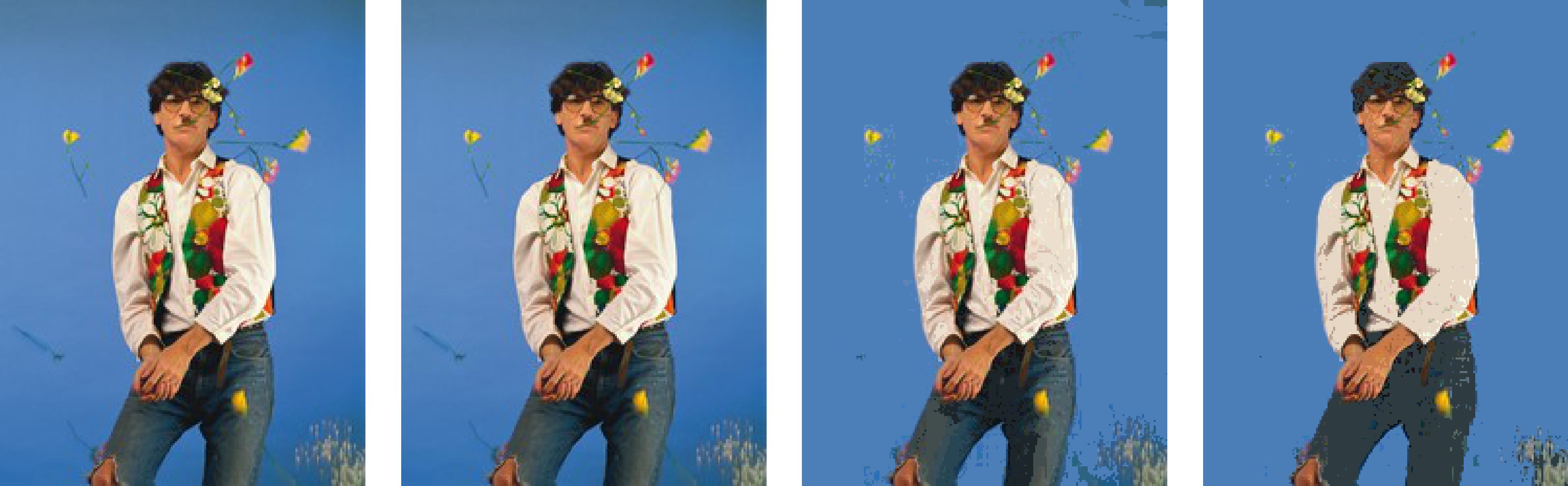
A small clustering can reduce the entropy without making the artifacts too noticeable. Also, we can get a huge reduction if we don’t mind the artifacts that much.
Linear algebra with images
Images in RGB format are just 3d arrays of values from \(0\) to \(255\). Thus it’s possible to see them as a subset of \(S=\mathbb{R}^{\text{width} \times \text{height} \times 3}\). We can define addition and multiplication by scalars in the natural way:
\[(A + B)_{ijc} = {A}_{ijc} + {B}_{ijc}\] \[( \alpha \cdot A)_{ijc} = \alpha \cdot {A}_{ijc}\]so this is a vector space and all the nice properties that it implies. A less pretentious way to see this is that we can flatten \(S\) to get ordinary \(\text{width} \cdot \text{height} \cdot 3\)-dinmensional vectors.
It follows that we can write any image as a linear combination with a basis of S. We should note that the elements that constitute this basis may or may not be images themselves as they can have negative values, non-integers or values larger than 255. Some basis are quite famous and a lot of fun effects are just simple modifications on a different basis. The heart of JPEG relies on using a good basis, but we are getting ahead of ourselves.
Suppose we decide to compress an image by erasing all information from certain pixels. We are not concerned here with how we encode the resulting image, just assume that we can. The reconstructed image is going to be kind of “uneven” in the sense that some pixels will be a complete representation of the original and some will have no relation to the original pixel at all. We can do tricks such as interpolating its neighbors to kind of hide it but this is no different than guessing. For all we know the pixel could be completely different than its surroundings.
With some imagination, we can see what’s happening when we remove pixels from a linear algebra point of view.
Let \(\boldsymbol C^{xyz}\) be the collection of elements from \(S\) that form the kind of “standard basis”.
\[(\boldsymbol C^{xyz})_{ijc} = \begin{cases} 1 & x = i, y=j, z=c \\ 0 & \text{otherwise} \\ \end{cases}\]Then the image pixel values are just the coefficients in this basis:
\[I = \sum I_{ijc} \cdot \boldsymbol C^{ijc}\]So, what happens when we erase all information from a certain pixel? This is simply removing the components related to \(\boldsymbol C^{ij1},\boldsymbol C^{ij2}\) and \(\boldsymbol C^{ij3}\). The rest of the components are unaffected. If we look at this phenomenon for a while, it’s obvious what is really going on: It’s a projection! Our “guessing” was just some fancy way to get values from \(<\boldsymbol C^{ij1} \boldsymbol C^{ij2} \boldsymbol C^{ij3}>\) (the orthogonal complement) that looked good enough. Naturally, erasing information from multiple pixels translates to removing more elements from the basis.
This perspective is really nice and leads to the following idea: Why should we stick with the standard basis when we can use any basis we want? That is, we can transform our image to a different coordinate system and then apply some lossy compression algorithm there. For example, we can pick some arbitrary linear subspace to project our image into and just store those coefficients.

That being said, there are some details to keep in mind:
-
Does our compression algorithm choose the basis depending on the image content? If it is image dependent then the header needs some extra information so the decoding part can work out the basis. On the other hand, if the basis doesn’t depend on the image content at all, no extra information is needed to know which basis was used.
-
How much precision do we want when storing the coefficients? Standard floats use 32 bits, this is 4 times more than the 8 bits of the RGB format. Clearly, we need to do something better than this.
The JPEG algorithm. Preamble
Now we try and implement JPEG, a real image compression algorithm (and a very common one that everyone uses). JPEG achieves such a high reduction in file size that it’s absolutely amazing. Its mechanism relies on exploiting deficiencies in how humans actually see (plus a good encoding).
The algorithm is a multi-step process with many moving parts. We will go through each, one by one, but in a nutshell, it goes like this: it applies two different transformations, each one followed by a lossy compression step, and then a lossless compression step in the end.
In JPEG, each transformation is a change of basis that is independent of the image so there is no header penalty involved in applying them. JPEG also has some adjustable parameters that control the amount of compression.
The JPEG algorithm. YCbCr Transform
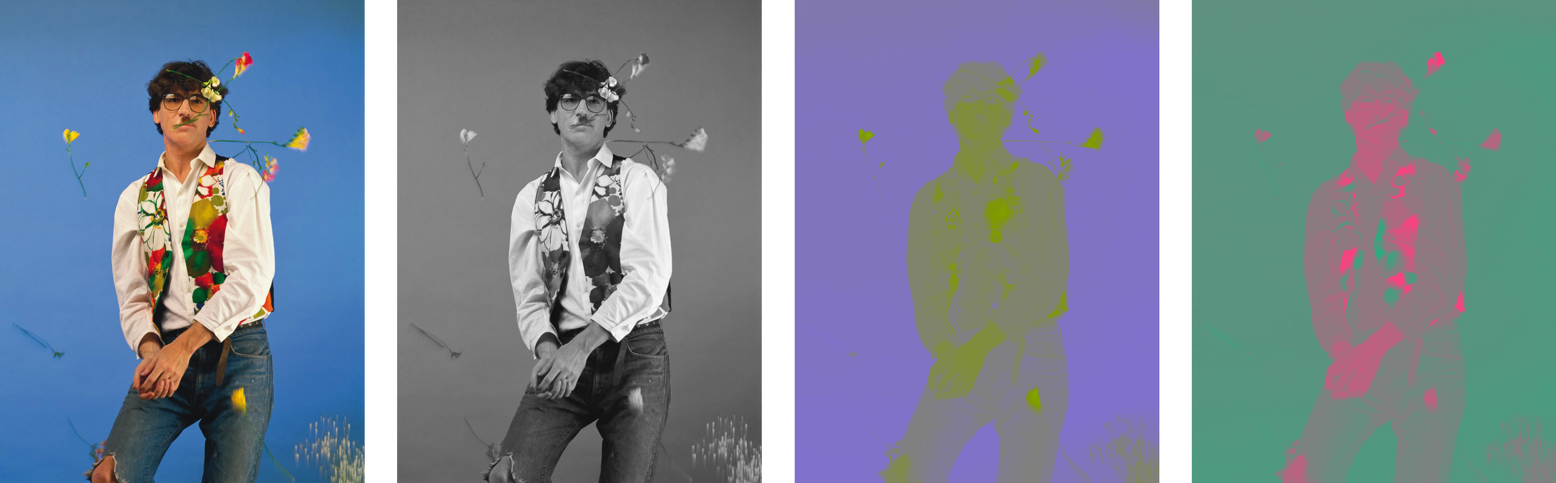
In the first step, we do a per-pixel transformation. Instead of using ranges of red, green and blue to indicate the pixel color, we use a different set of components called luminance (Y), blue chrominance (Cb) and red chrominance (Cr).
Luminance ranges from black to white. Blue chrominance ranges from yellowish green to purple. Red chrominance ranges from light green to pink.

Each value is just a linear combination of the RGB values so, in the end, this is just a change of basis, as we have seen before5.
After doing this transformation we do some lossy compression. The intuition is that while our eyes are good at detecting changes in brightness, we don’t really see color all that well. For this reason, it’s possible to reduce the quality of the chroma channels without it being noticeable. More precisely, after separating the components, we subsample the chroma channels, reducing the amount of rows and columns (for example discarding/averaging across multiple rows/columns). The common subsampling for JPEG seems to use one sample per 2x2 block for the chroma channels. Just by doing this we get a nice reduction to 12 bits per pixel. We should note however that the subsampling part is not particularly powerful, it doesn’t reduce the file size that much, at least compared to the following steps. If we wanted to, we could skip the subsampling without significantly affecting the compression.
The JPEG algorithm. Cosine Transform
From the last step, the image has been separated into Y, Cb and Cr. Now comes a more complicated transformation. In short, the basic idea is grouping the channel array into nxn blocks and then using cosine transforms to separate each block into its spatial frequencies. Cosine transforms are similar to Fourier transforms but they use only cosine waves as their basis instead of complex exponentials. The basis elements \(\boldsymbol A^{k_1k_2}\) for the nxn blocks are:
\[(\boldsymbol A^{k_1k_2})_{ij} = \bbox[5px,border:2px solid red] { \alpha(k_1) \cdot \cos \left( \frac{k_1 \cdot \pi \cdot ( i + 1/2)}{n} \right) } \cdot \bbox[5px,border:2px solid blue] { \alpha(k_2) \cdot \cos \left( \frac{k_2 \cdot \pi \cdot ( j + 1/2)}{n} \right) }\]The alpha multipliers just act as scaling constants. We could use any scaling constants we want (naturally, this will affect the coefficients we get after applying the transformation). In our implementation we use \(\alpha(0) = 1\) and \(\alpha(x \neq 0) = 2\). As far as I know these are not the ones that JPEG uses but they are simple and seem to work well in practice.
The equation for the basis elements \(\boldsymbol A^{k_1k_2}\) looks complicated but it’s actually pretty simple. \(\boldsymbol A^{k_1k_2}\) is just the multiplication of two waves. One of them is traveling in the \(i\) direction with a frequency related to \(k_1\) and the other one is traveling in the \(j\) direction with a frequency related to \(k_2\).
With 8x8 blocks (JPEG uses \(n=8\)) we get the following basis elements:
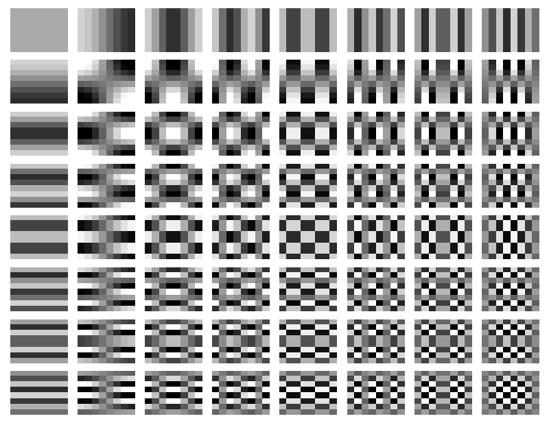
Notice how you get the interior elements by multiplying one element from the first row and one element from the first column (and multiplication by a constant because of the different alphas).
Anyway, after the cosine transform each value in the block is the coefficient of the related spatial frequency.
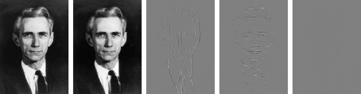
From left to right: original, only the (k1=0 k2=0) components, only the (k1=0 k2=1) components, only the (k1=1 k2=0) components, only the (k1=1 k2=1) components.
Now we do quantization. Basically, we transform each coefficient from real numbers to integers. In the quantization step the real line is split into pieces of the same length and then an integer is assigned to each one. If a number falls in a range with assigned integer \(x\) then it is quantized to \(x\). As this is true for any number that falls within the same range, you can’t recover the original value you had before the quantization. Of course, the smaller the pieces, the higher the precision that we get.
The trick is that in real images the higher frequencies tend to have close to zero coefficients so they don’t contribute much to the image 6. Besides, our eyes don’t pay much attention to these subtle higher frequencies effects anyway. With that in mind, we can use less precision when storing those coefficients. In more formal terms, our quantization does the following: given block \(\boldsymbol B\) and quantization table \(\boldsymbol Q\):
We just need to use larger values in the higher frequency entries of \(\boldsymbol Q\) and we are done.
The mechanism by which one comes up with the exact values to use in the quantization table \(\boldsymbol Q\) is way beyond my understanding. There seems to be a lot of different tables. In the end, (I think) these tables are just trying to put numbers on the way humans see images. Also, different tables are used for the luminance and chrominance channels. As we have said before, we don’t see color all that well so we can use bigger quantization for high-frequency coefficients in the chrominance channels. Another feature is that quantization tables can be multiplied by a constant so as to control the quantization precision. For instance, if we multiply the tables by \(0.5\) we would halve the piece’s lengths and preserve a higher level of detail.
The quantization step, done after the cosine transform, is responsible for most of the lossy compression and is the central part of the algorithm. Grouping values into the same integer is going to result in the most compression later when doing the lossless compression step. One can view the quantization as a form of clustering. Similar to the example of clustering colors, combining symbols reduces entropy so it will help when doing entropy encoding, specially considering that most high-frequency coefficients are going to be zero after quantization. In addition to reducing entropy, sequences with large runs of the same symbol are great for performing run-length encoding, as we will show next.
The JPEG algorithm. Run length and Huffman encoding
The last step of the algorithm is the lossless compression step. First, let’s talk about run length encoding. Run length encoding transforms a sequence of symbols into a sequence of (symbol, count) pairs. The count indicates the amount of consecutive appearances. It’s easier with an example:
\[AAABBCAA \xrightarrow{\text{run length code}} (A3)(B2)(C1)(A2)\]If your strings tend to have large runs of the same symbol repeating over and over then this trick might help reduce the string size.
Now, going back to what we have from the last step. After quantizing the channels, we ended up with three arrays in which many close values were mapped to the same integer, mainly in the higher frequencies. We need to flatten the arrays so that we can see them as a stream of symbols, just like in color encoding, and perform some lossless compression tricks. However, does every flattening work equally well? If we only want to use huffman encoding then yes, we really don’t care about how we flatten the array. The performance of techniques like huffman encoding doesn’t depend on the order of the symbols, just on the symbol distribution. On the other hand, run length encoding does depend on the order, it needs large runs to work well. So, if we are going to use this last encoding, we better try to create large runs when flattening.
The way that JPEG does this is that it zig-zags through the frequencies. By doing this, we get a large run of 0s since the higher frequencies are going to be stored together.

This is not the full story. There are other complicated processes in the lossless compression part of JPEG. JPEG separates the flat frequencies coefficients (the ones with k1=0, k2=0) from the rest and does something called Differential Pulse Code Modulation, I have no clue what that is.
This is the part that we diverge significantly from JPEG. From here on, this is our custom version.
We implement a much simpler lossless compression step that seems to work well enough. First, we don’t separate the flat coefficients. Second, instead of zigzagging through the block, we zig-zag through the whole array but only looking at one frequency at a time. That is, first we zig-zag the array, collecting all flat coefficients, then we switch to another frequency and repeat the process and so on. We hope that, when collecting all coefficients of some high frequency, we still get some large runs of 0s.
After doing this flattening, we concatenate the one-frequency sequences and so we end up with three flat arrays (one for each channel). Then we apply run length encoding to each one and separate the (symbol, count) sequences into two different sequences: one for symbols and one for counts. Finally, we do huffman encoding to each of the three symbol sequences. This last step will add three codebooks to the header.
The JPEG algorithm. Putting it all together
We have all that we need. To summarize everything we’ve done in our slightly off JPEG implementation:
- YCbCr transform
- Subsample the chroma channels
- Cosine transform
- Quantize using quantization table
- Flatten channels trying to get large runs of 0s
- Run length encode each channel
- Huffman encode the symbol components of the run length codes
Again, there’s still a lot of low-level stuff involved in the implementation. Look at the repo for more details about how this is done.
Now that we have our custom JPEG, we can test how well it works. We sample images from picsum and look at the bits per pixel used. There’s also the quantization table multiplier that we can play with. Smaller multipliers lead to less compression but a greater similarity to the original image. So, sampling 700 images for a couple of quantization multipliers, we get the following:
Clearly, we are doing much better than the 12 bits per pixel of color coding. The fact that we can compress the image so much that it only needs a few bits per pixel is unbelievable. For instance, look at the following:
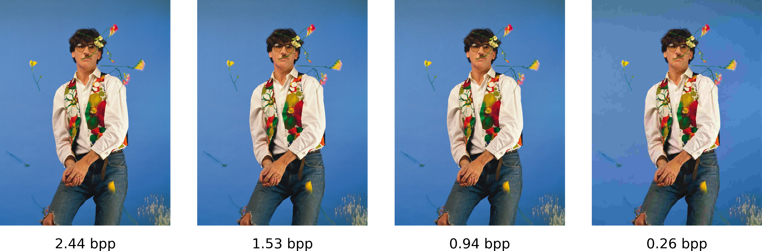
Remember, we began with 24 bits per pixel! With our custom JPEG, even using a small quantization multiplier, we end up using less than 3 bits per pixel and the image still looks really well. Not to mention, we were kind of sloppy in the lossless compression part and we still managed to greatly compress the image.
The thing that still amazes me is that looking at the images it definitely doesn’t feel like they carry so little information per pixel. But they do. Pretty cool, right?
Footnotes
1: As another fun example, neural networks for computer vision have a problem in which a small modification in an image can change a neural network output while being unnoticeable to the human eye. See here.
2: Talking about the distribution of real images is not completely valid. The kind of images we send changes through time. It’s more like a random process. We are simply ignoring that. That being said, it does not change that much. We can safely assume that images of humans are still going to be common in fifty years, even though it may not be the same faces that we are familiar with.
3: Tom Scott explains Huffman codes really well in an amazingly short time. See here
4: To be fair, it depends on the image size. More pixels imply a smaller overhead per pixel (although bigger images may use more colors). For 1024x1024 the bits per pixel used was much closer to entropy.
5: Some implementations add a constant to the Cb and Cr components. This shift, strictly speaking, stops it from being just a change of basis.
6: Some images (such as those containing text or things with lots of edges) do have a large contribution of high frequency coefficients. Their effect on the image is not subtle. In those situations, artifacts are going to be more noticeable.
References
- The wikipedia page on JPEG is the main source for the JPEG part.
- JPEG DCT, Discrete Cosine Transform - Computerphile. See here. All their videos on JPEG are really good
- This link gives a brief overview of all the steps involved in JPEG.
- Thomas M. Cover and Joy A. Thomas. 2006. Elements of Information Theory. For the short information theory related discussions. Only the first few chapters.