How to build NVAE from scratch

This is just based on my attempt to understand NVAE’s original code, there is no guarantee that it is correct. I made my own implementation, and it seems to work (more or less), so I hope I’m not too far off.

Introduction

There’s a paper from 2021 called NVAE. A Deep Hierarchical Variational Autoencoder. It aimed to “make VAEs great again” with an architecture called Nouveau VAE (NVAE) that generated high-quality images using a VAE approach. It was pretty cool as VAEs typically perform worse than GANs for image synthesis. While NVAEs are a step forward for VAEs, they still have some issues. They use a lot of GPU memory and, as a consequence, it’s only feasible to train them for smaller resolutions and using a small batch size.

The original code (see here) is somewhat messy to follow ¹. I tried reproducing the NVAE architecture myself by looking at it. It was a struggle, I don’t think I’ve completely succeeded. In this post we give (most of) the needed steps to recreate the NVAE architecture if you want to do it yourself. A sort of NVAE Cookbook if you will. I should point out before continuing that the code has multiple possible tweaks and alternative architectural components here and there. I focus only on one of them, trying to follow the versions that are used on the training examples on the repository. There are a couple of low level tricks that I ignore here. I’m concentrating mostly on describing the structures. You can also see my implementation here with all the details.

As it usually happens with this sort of things, it’s easier to understand some architectural feature by showing a diagram than by reading about how a group of components is intertwined in some complicated relationship. Because of this, I’m strongly relying on diagrams I made on Inkscape to convey most of these features. Hopefully, it’s going to make things more understandable.

Also, note that the names for referring to different parts of the architecture are mostly non-standard so bear that in mind when reading the original paper and not finding words like “mixer” in there.

General structure

Here is a rough road map of NVAE’s architecture:

During training, the initial \(X\) is preprocessed and then it goes through the encoder tower. The encoder tower outputs a series of tensors of different sizes. As you advance in the encoder tower you would reduce the dimensions and increment the channels progressively.

For example, you may have that the encoder tower outputs tensors with shapes:

20 x 64 x 64, 20 x 64 x 64, 40 x 32 x 32, 40 x 32 x 32, 80 x 16 x 16

Each of these tensors goes to the mixer. The mixer is in charge of generating the latent variable \(z\) based on an input from the encoder tower and an input from the decoder tower. Each \(z\) follows a gaussian distribution.

Each block in the decoder towers receives an input that depends on both the output from the previous decoder block and the previous \(z\). As you can see in the diagram, the blocks in the decoder tower follow an opposite direction than the ones in the encoder tower. That is, the first output from the encoder is mixed with the last output from the decoder and so on. As you advance in the decoder tower, you copy the behavior of the encoder tower “in reverse” by incrementing the dimensions and reducing the channels accordingly.

After that, you go through a round of post-processing and end up getting the parameters of a mixture of clipped logistics for each pixel. This is the final distribution that you are going to sample your reconstruction from.

Encoder cells and blocks

The encoder tower is made out of encoder cells organized in a certain way. Each of these cells follows a residual pattern.

You put a series of these residual cells back to back (how many is determined by a hyperparameter) to form an encoder block. The input goes through this residual chain and then what comes out of it is broken into two copies. One copy ends up going to the next encoder block and another copy goes to the mixer.

When an encoder block performs a downscale, an extra encoder cell is added at the beginning of its residual chain. This extra cell performs the downscaling.

Encoder Tower. How are blocks grouped

We use some hyperparameters to determine how many splits we should perform before downscaling. This is done with exponential decay. You start with some initial_splits number of splits and after you downscale, you divide this by a constant (usually 2) and use that number of splits and so on. All of these blocks that go sequentially before the downscaling constitute a group. A hyperparameter indicates the number of groups in the encoder tower.

Here is an example. Suppose that the initial input to the encoder tower has shape 20 x 64 x 64, initial_splits=8, the decay factor is 2, and that our encoder tower has 3 groups. The encoder tower is going to output the following shapes to the mixer:

• 8 tensors of shape 20 x 64 x 64,
• 4 tensors of shape 40 x 32 x 32,
• 2 tensors of shape 80 x 16 x 16

We can also flatten the decay by having a minimum number of splits that a group may have.

Decoder cells and blocks

The decoder cells have a different set of components than the encoder cells, but the basic structure remains the same, a residual pattern. They look like this:

They are grouped much like the encoder cells. You put a series of these residual cells back to back (with another hyperparameter) to form a decoder block. The input for the blocks comes from the mixer output of the previous level. After going through this residual chain the output is taken as the input for the next mixer block.

When a decoder block performs an upscale, you add an extra decoder cell at the beginning of its residual chain. This extra cell performs the upscaling (you add a bilinear interpolation before going through the sequence of layers).

Decoder Tower

As we have said before, the decoder tower is structured to mimic the encoder tower. In other words, the number of groups and the size of each one of these is already determined.

A tricky part is to figure out where exactly should the upscaling blocks be. The decoder tower goes in reverse and the tensor’s shape from this decoder block should be the same as the one coming from the encoder block so, how do we do this?

The solution is that a decoder block should upscale if the next block from its encoder pair is a downscale. The reason behind this is that the upscale is “reversing” the change in shape caused by the next downscale block. It sounds messy but here is an example:

Mixing Block

The mixing block combines the output from the encoder block with the output from the decoder block. The mixer outputs the tensor you are going to use as the input for the next decoder block.

The mixer block is also where the sampling of the latent variable \(z_i\) happens. This process involves taking the input tensor in \(\mathcal{N}\) as a pair of parameters: \(\mu\) and \(\log \sigma\). These are going to be used to sample from the gaussian distribution.

Now, the first mixing block is slightly different. Here the tensor we get from the decoder is actually a learnable constant. In this situation, the decoder input is not involved in the \(z\)-generating process. The encoder tensor is the only one that contributes to the gaussian parameters while the decoder tensor goes straight to concat. At sampling time we don’t have an input from the encoder so we use \(\mathcal{N}(0,I)\) instead.

We should also note that each \(z_i\) may not have the same shape. Each \(z_i\) inherits its width and height from the encoder/decoder tensors and its number of channels from a hyperparameter latent_channels.

Continuing our previous example, with latent_channels=7 we are going to have the following shapes for the \(z\)s

• 8 tensors of shape 7 x 64 x 64,
• 4 tensors of shape 7 x 32 x 32,
• 2 tensors of shape 7 x 16 x 16

Mixer block during sampling and KL loss

The mixing procedure is obviously modified when generating new images as there are no tensors coming from the encoder. When sampling our VAE, we remove two sections. First, we remove the upper part of the process that is involved in creating the gaussian distribution. Meaning that our parameters for \(\mathcal{N}\) are going to come straight from the ELU+Conv2d part. The other part we remove is the normalizing flows block. That is, after getting \(z\), we skip the normalizing flows block and take \(z\) directly to concat.

The KL loss is going to be between the \(z\) generated after going through the normalizing flow and the one that would be produced using only the decoder part. As \(z\) goes through the normalizing flows it abandons its original gaussian distribution. Because of this, we can’t actually use the closed form of the KL-divergence between gaussian distributions. So, we rely on empirical values. That is \(\log p_{\text{mix}} (z_{\text{mix}}) - \log p_{\text{decoder}}(z_{\text{mix}})\)

Note that, even though \(z_{\text{mix}}\) is not gaussian, we still know \(p_{\text{mix}}\) because of how the normalizing flow block transforms the random variable.

Normalizing Flow Block

I don’t want to dwell on the inner structure of the normalizing flow too much because it is highly likely that I misunderstood part of it but here it goes. Each normalizing flow block consists of a series of pairs of normalizing flow cells. The exact number is determined by a hyperparameter. Each cell looks like this:

They are paired because there is a small difference between the first cell in the pair and the second one. You mirror the convolutional mask of the Autoregressive Conv2d for the second cell. To understand what we mean by this, we must talk a bit about the autoregressive convolution. Basically, you apply a mask to each kernel before performing the convolution. The masks look like this:

So, the cells alternate: one that only takes input from before values, one that only takes input from after values and so on.

In my experience, you can also get good results without using normalizing flows at all. So, it doesn’t seem to be that important. Plus, if we don’t put \(z_i\) through the normalizing flow we can use the closed form of the KL-divergence between gaussians!

Preprocess

The preprocessing of the input is very simple. We start with an image \(X\) from the dataset, and then we apply:

1. A 3x3 convolution that switches the number of channels from the original 3 (rgb) to channel_towers, a hyperparameter.
2. A series of downscaling encoder blocks. The number of cells per block and the number of blocks are determined by hyperparameters

Postprocess

The postprocess is similar to the prepoccess in reverse

1. A series of upscaling decoder blocks. The number of cells per block is determined by a hyperparameter. Here the number of blocks is going to match the amount we used for the prepocessing. There is one small difference between residual cells in the postprocess and in the decoder. In the decoder we use a hidden channel multiplier of 6 while in postprocess we use 3.
2. ELU+Conv2d 3x3 that switches the number of channels to \(d\) where \(d\) is the number of channels we are going to use in our final distribution.

For example, if we use a per subpixel gaussian distribution we are going to have \(d=6\) as 3 channels are going to \(\mu\) and 3 to \(\log \sigma\). If we keep the variance constant we may reduce this to \(d=3\) as we did previously (see here) but that would probably give worse results.

NVAEs use something called discrete logistic mixture. It is a somewhat complicated distribution. In the next section we go into more detail about it.

Discrete Logistic Mixture

NVAEs use a mixture of discrete logistics at a subpixel level ² as their final distribution. There’s a hyperparameter n_mix indicating the number of distributions in the mixture. Each of these distributions has 2 parameters: one for the mean and another one for scaling. They are defined on the (-1,1) range ³ so after taking our samples we apply a shift using \(\frac{x+1}{2}\).

Here is a more detailed explanation. For each pixel, we randomly pick index \(K_{ij} \in [1, \text{n_mix} ]\). This uses n_mix parameters per pixel to define the probability of picking each one. Then, this chosen index \(K_{ij}\) is used to decide which of the per-channel logistics to sample from. It’s important to note that while each pixel channel has its own set of logistics, all 3 of them share the same random variable \(K_{ij}\). Each subpixel distribution in the mixture is a clipped and discretized version of the logistic distribution. We can see it as applying 2 transformations on a logistic distribution.

1. \[Z_{cijk} \sim \text{Logistic}(\mu_{cijk}, \text{scale}_{cijk})\]
2. \[Z^{\prime}_{cijk} = \text{clipped}(Z_{cijk},-1,1)\]
3. \[Z^{\prime\prime}_{cijk} = \text{round}(Z^{\prime}_ {cijk}\cdot 256) / 256\]

In short, using these random variables we have that the per-pixel image distribution is:

Luckily, we don’t need to discretize during sampling as the output is already mapped to the closest color when displaying images. However, must take it into account when calculating \(\log p(V_{cij} = x)\)

The original implementation also includes n_mix extra parameters to perform some autoregressive transformation of the RGB channels ⁴.

Our implementation actually differs here by skipping this last step. We also use a per subpixel selector random variable instead of having the same selector for all pixel channels. That is, we use \(K_{cij}\) instead of \(K_{ij}\). It seems to work on practice.

Trick 1. Readjusting batchnorm

Neural networks with batch norm layers have different behavior at training time and at evaluation time. ⁵. During model evaluation, you use a running average of the statistics obtained during training.

This paper does the evaluation slightly different. Here, before freezing the batchnorm layers, you take a bunch of samples in order to move the running average. Once you have adjusted these statistics, you freeze them up and take the “real sample”. This seems to increase image quality and diversity. I can only imagine this discovery was the result of someone forgetting to put the .eval() at sampling time.

The downside is that sampling is going to be slower. And, as these new running averages depend on your sampling temperature you can’t do it once and leave it at that (unless, of course, you also leave the temperature fixed).

If you use too many iterations the quality starts to deteriorate. There’s a lot of trial and error. Ultimately, the number of iterations you should use seems to be more art than science.

Trick 2. Balancing KL losses

Handling the KL loss during training with this architecture requires sort of a delicate balance. It’s very common to find that the KL loss falls down to almost zero in some parts of the tower (in my experience it tends to be the first groups). That is, the decoder contribution to the encoder-decoder mix is mostly non-existent.
This usually indicates that those parts of the network aren’t actually transmitting any information down the tower so they end up being useless. They still contribute to the size of the network and the speed of training so they act as “dead weight”. The paper’s approach to solve this problem is to have different KL loss multipliers during the KL warm-up. The process is a little bit more involved but in short, smaller spatial tensors have a smaller KL multiplier to diminish the pressure they have and thus avoid this phenomenon.

Some samples and training information

Ok, finally we show some results of our custom implementation. Replicating the architecture parameters of the paper is not possible as it requires a lot of memory (and a fast GPU). We use the following small-scale hyperparameters for a 64xx64 version of the ffhq dataset:

channel_towers: 32
number_of_scales: 3
initial_splits_per_scale: 6
exponential_scaling: 1
latent_size: 20
num_flows: 0
num_blocks_prepost: 1
num_cells_per_block_prepost: 2
cells_per_split_enc: 2
cells_per_input_dec: 2
n_mix: 10

It’s a small model, around 150MB. Note that there are no normalizing flows here. I wasn’t able to get good results using them but this is probably due to a bug in the implementation.

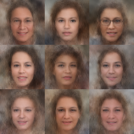
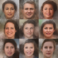
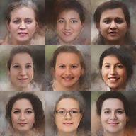
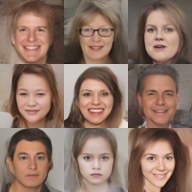
It takes roughly 4.1 GPU days to get nice results⁶. Here are some cherry-picked samples at a low temperature.

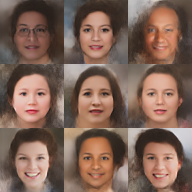
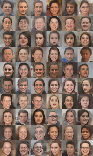
Here are some non-cherry-picked samples:

I should also note that there’s another implementation of NVAE here that gets much better samples using a smaller architecture so there’s likely some other issues with our version.

References

• NVAE: A Deep Hierarchical Variational Autoencoder by Arash Vahdat, Jan Kautz
• Github repo of the official pytorch implementation of NVAE
• Pixelcnn++: improving the Pixelcnn with discretized logistic mixture likelihood and other modifications” by Tim Salimans, Andrej Karpathy, Xi Chen, Diederik P. Kingma
• Improving Variational Inference with Inverse Autoregressive Flow by Diederik P. Kingma and Tim Salimans and Max Welling
• Squeeze-and-Excitation Networks by Jie Hu, Li Shen, Samuel Albanie, Gang Sun, Enhua Wu

Footnotes