An original rambling of mine with minimal hope of coherence. Most discussion here is not based on any set of papers, particularly the Markov chain exploration. It’s quite likely that it is wrong so be aware of it. It seemed interesting, so I may as well share it.
What’s super-resolution?
Super-resolution is about taking an object with certain resolution and outputting a version of it as if it were of a higher resolution. It takes an object with some information content and guesses a bit more of what it’s given. Its job is to create (not deduce) a plausible version of said object with more information. While this all sounds very fancy, there are a lot of straightforward examples. For instance, a super-resolution algorithm may be concerned with scaling a 64x64 image into a 256x256 image. Variations of this application are very fashionable these days, being used for increased performance in games link or on the pipeline of text-to-image models link.
It’s cool and it denotes how little information is conveyed in real images 1. The information content of an image is much less than what seems natural at first sight because the real world behaves in some very precise ways and as a consequence, even though image space is enormous, most of it doesn’t align with our perception and experiences. Therefore, a good super-resolution algorithm requires some knowledge of the real world (and how we see things) to arrive at a reasonable outcome. There is only a subset of valid possibilities. Take the following related example:
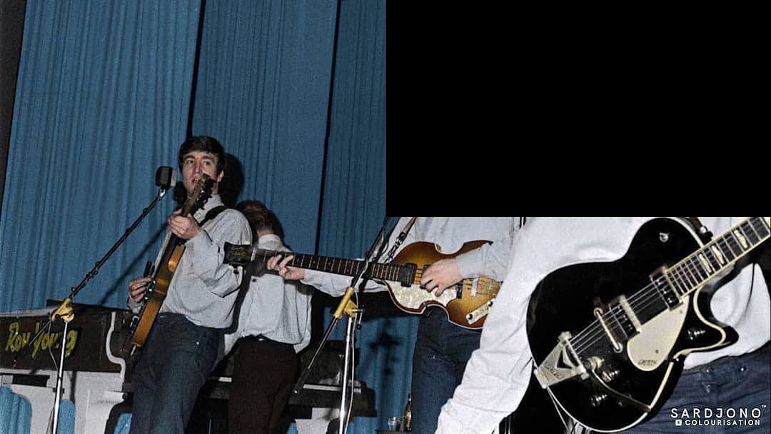
Image source.
To complete the image reasonably it needs to know that it’s a photo. Any random noise won’t work. More than that, it needs to understand that the blue background is likely to be present. How humans look like. That this is a band. That it’s the Beatles. That Paul plays bass and George plays guitar, and so on. No patch-filling method is going to work well without some understanding of the input distribution. The same goes for super-resolution algorithms.
Markov chain setup
We can actually cast this problem into familiar information theory terms for the discrete case. Whether such an interpretation is fruitful or not is a different issue. It’s certainly fun to interpret these things using these concepts.
We can imagine the input playing the role of the “real world” generating the full-resolution object. However, we on the decoder side have no direct access to this. Our “sensor” sends us a low-resolution object conditioned on the input. This is then sent to our receptors that infer a message (basically our brains) based on it.
Ideally, our sensor would be transparent. That is, it would identically retransmit its input. But, we have no control over the receptor, so we add a machine between sensor and receptor that approximately “autocorrects” it 2. The objective of the decoder is not to truly obtain a high-resolution reconstruction but to make the receptor interpret the same message as if its input were of high-resolution. Note that the transmission protocol is fixed from the start as nature plays both the side of the transmitter and the sensor. We can only decide how the decoder operates. This model seems quite general and can work for different kinds of problems such as super-resolution or patch-filling.
The existence of the receptor may require further clarification. The purpose of this high-resolution object is to be used by the receptor. It doesn’t matter what the receptor receives as long as it interprets the result correctly. For example, you can mess up an image quite a bit before people start to notice. Another option is to replace the receptor with a perceptual loss that measures how much the reconstruction differs from the original high-resolution version, but we’ll talk more about it in short.
We introduce a couple of definitions for random variables.
- \(HR\) as the high-resolution.
- \(LR\) as the low-resolution.
- \(SR\) as the decoder output.
- \(\hat{M}\) as the message interpreted by the receptor going through all the steps
- \(M\) as the message interpreted by the receptor if it came straight from the high-resolution.
We then define the following chain:
\[M \rightarrow HR \rightarrow LR \rightarrow SR \rightarrow \hat{M}\]The true message generates the high-resolution object. The sensor transforms it into a low-resolution version. Then it goes through the decoder and to the receptor to be interpreted as a message.
The mutual information \(I(LR,M)\) quantifies sort of an upper limit on the amount of information that we’ll be able to squeeze about \(M\) out of the low-resolution version if we are lucky.
In the extreme case where the \(LR\) contains all information about \(M\) then it’s clear what we should do. We can actually figure out with complete certainty what message \(M\) the receptor should get. We can then make our decoder generate something that guarantees \(M = \hat{M}\). In short, the decoder should simply output any high-resolution object that leads to \(M\) (such existence is guaranteed because \(H(M\mid LR) = 0 \implies H(M\mid HR) = 0\)).
Now, for the more complicated case of a \(LR\) that drops bits, it is not so clear-cut. The problem is ill-posed. We don’t completely know \(M\). The decoder must make an educated guess about the intended message and output something accordingly. Naturally, we not only want to preserve all/most information we already have about \(M\) but also attempt to make \(M = \hat{M}\) (these are not the same thing !3). It’s interesting that, if we assume that \(\hat{M}\) has the same distribution as \(M\), then we are generating \(H(M \mid LR)\) bits (on average) at the decoder. That’s our extra information! I think it’s pretty cool that, at least theoretically, we can formalize this intuition about the information that is invented at the decoder.
There are some caveats to this elegant interpretation. Mainly, if \(LR\) has some extra randomness (\(H(LR) > I(LR,M)\)) then those extra bits might be technically coming from there and used by the decoder as “random fuel”. It’s sort of deriving meaning from the noise. And even so, in problems such as super-resolution, the downsampling is deterministic so all extra bits are created by the decoder. But we may also argue that \(\hat{M}\) does not need to follow the same distribution and so the decoder can simply work with what is given and not create extra randomness. It’s also important to note that this is a statistical property. \(LR\) might sometimes have no information about \(M\) and sometimes have a full description. The same goes for the decoder. It may sometimes heavily rely on the original message and sometimes it might create something unrelated.
Another interesting property derived from this setup is that, in the discrete case, if both the sensor and the decoder are deterministic then (unless we have a sensor that preserves information) we won’t be able to emulate that amount of information using \(\hat{M}\). The output distribution will always be less “rich” 4.
But, is imitating the distribution while keeping the mutual information always possible? I’m not entirely sure, although I suspect that it is. This is true at least when we have access to the full message \(M\), but I don’t know for the case of only seeing a random variable that shares the information.
Anyway, based on this model for the setup, we need to figure out what objective should we minimize when guessing if we can’t completely know \(M\). A plausible definition for a minimization objective is:
\[E[D[M \mid LR \| \hat{M} \mid LR]]\]With \(D\) being some statistical distance (well, not necessarily a distance but you get the point). Plus, as a byproduct, this setup merges well with generative models. Generative models can be interpreted with this definition. Generation is simply having a really bad sensor. That is, \(I(LR,M) = 0\) and thus \(D[M \mid LR \| \hat{M} \mid LR] = D[M \| \hat{M} \mid LR]\). Inversely, problems such as super-resolution are, if you think about it, simply conditional generative models.
I’d like to restate that this minimization objective is not in any sense special or important. It’s just a general theoretical construct.
The problem with perception. Surrogate objectives.
While I think this setup is cool, there’s a fatal flaw. How do we know the final messages? There is no real way to get the receptor output in most human-centric problems5. Both \(M, \hat{M}\) are completely inaccessible to us. Essentially, how do we know what goes through someone’s mind while seeing an image?
To be fair, yes, there are some approaches to conjure some complicated perceptual loss that somehow mimics human perception, but they are guesses nonetheless. The interesting part, at least to me, resides in the presentation of the model itself. There are other reasons why we may not use the messages such as being too slow to obtain or being private property.
So anyway, what shall we do then? Well, we use a surrogate objective. There are multiple techniques.
Take \(d_h\) to be a distance function in image space and \(d_s\) to be a distance function in message space. Take \(s\) to be the function playing the role of the receptor mapping from image space to message space. If we assume that \(s\) is Lipschitz continuous for these distance functions then
\[E[d_s(M, \hat{M}) ] = E[d_s(s(HR), s(SR)) ] \leq k E[d_h(HR, SR) ]\]for some \(k>0\). That is, this loss works as an upper bound. We don’t even need to know \(d_s\). We just need to hope that this property holds for some sensible unknown distance function. This may not be a reasonable request sometimes. It imposes some requirements on message space that we truly don’t know. Minimizing losses such as MSE are typical for “vanilla” approaches6 but you don’t have to. Some incorporate the fancy perceptual losses coming from neural networks.
Other techniques more in line with the objective mentioned in the previous section use a more statistical approach. Given an \(f\)-divergence then the following property holds:
\[D[M \mid LR \| \hat{M} \mid LR] \leq D[HR \mid LR \| SR \mid LR]\]Thus, we can try to optimize the \(SR\) distribution which bounds our true objective. Classic GANs go here, as they are minimizing the Jensen–Shannon divergence. Max likelihood methods such as VAEs are also in this category as they are minimizing (a bound on) the Kullback-Leibler divergence.
Side proof
Random variables sharing information
Given a random variable \(X\) and a \(\beta \in [0,1]\) there is a random variable \(\hat{X}\) such that \(I(X,\hat{X}) = \beta H(X)\) and \(X \stackrel{d}{=} \hat{X}\).
To prove it we construct such \(\hat{X}\). Take \(E\) to be a Bernoulli with probability \(\beta\) and \(X_2\) an independent variable with the same distribution as \(X\).
\[\hat{X} = \begin{cases} X_2 &\quad\text{if } E=0\\ X &\quad\text{if } E=1\\ \end{cases}\]It’s clear that \(X \stackrel{d}{=} \hat{X}\). Now for the mutual information we have that
\[H(\hat{X} \mid X) = (1-\beta) H(X)\] \[I(\hat{X}, X) = H(\hat{X}) - H(\hat{X} \mid X) = \beta H(X)\]References
- Perceptual Losses for Real-Time Style Transfer and Super-Resolution by Justin Johnson, Alexandre Alahi and Li Fei-Fei.
Footnotes
-
Even only using standard lossy compression algorithms it’s possible to send less than 1 bit per pixel without significantly altering an image. I talk about it here. ↩
-
Another modeling option is to put the decoder before the sensor so that it directs the sensor behavior. Just like you put glasses before your eyes. ↩
-
For example, take \(X \in \mathbb{R}\). Clearly \(I(X,X+1) = H(X)\) but \(X \neq X + 1\) ↩
-
Richness might be a bit theatrical. Basically, it will have less entropy. ↩
-
There are multiple examples showcasing the difference between what’s in an image and what you see in an image. A fun recent one is a paper on the artifacts on CNN-based generative models. ↩
-
There might be a strong theoretical argument that justifies L1 or L2 losses that I’m not aware of so take it with a grain of salt. I believe that, while such losses are very intuitive, as long as the objective is human visualization, they are ultimately relying on the hope that it will look good. ↩