Variational Autoencoders Notes

I’m out of my depth here but I was curious enough about the subject to explore it. My probability background is not particularly strong, so these notes might be too simplistic and not reflect all the subtleties and interesting ideas involved

VAEs and the generative modeling landscape

Variational autoencoders are a kind of neural network architecture for generative modeling. They work by using some clever math and (at the time of writing) they are one of the main competitors to GANs in the domain of image generation. One of the advantages that VAEs have over GANs is that they seem to give more diverse samples¹.

We’ll go through some related concepts, talk about the main idea of ​​VAE, and finally we’ll do a simple implementation in PyTorch.

Setup

Our objective is to emulate the random variable \(X\) following an unknown distribution \(p\) given a set of samples. It goes without saying that whatever method we end up using in order to achieve this, we ultimately want to generalize beyond the training examples that we feed it instead of regurgitating data.

We start from \(Z\) following a distribution \(u\) we do know. If we apply a function to \(Z\) we can shape the distribution to resemble \(p\). Take \(f_\theta\) to be the parametrized function and \(p_\theta\) the associated distribution. That is:

So, we are searching for a \(p_\theta\) similar to \(p\). An intuitive method for picking a \(p_\theta\) from the parametrized family is optimizing \(\mathbb{E}[\log p_\theta(X)]\), the expected log-likelihood. Assuming that \(f_\theta\) is continuous on \(\theta\) (like a neural network) then we could use gradient ascend with the gradient \(\nabla \mathbb{E}[\log p_\theta(X)]\). The catch is that if \(f_\theta\) is too complicated then it’s going to be hard to calculate it, at least analytically. Also, as we will show next, using a plain neural network for \(f_\theta\) doesn’t work.

A plain neural network for \(f_\theta\) doesn’t work

The problem with directly using a neural network is that \(p_\theta(x)\) is going to be 0 at the beginning of training for any \(x\) taken from the dataset ². We assume that \(f_\theta\) is continuous in \(\theta\) so small changes won’t lead to any \(z\) mapping to \(x\). So \(p_\theta(x)\) doesn’t change at all. There is no training signal! ³. Oversimplifying, taking the network as our generator correlates with an “all or nothing” approach. Either it copies samples from the dataset or it doesn’t.

Clearly, we want to gradually push the network to produce outcomes more and more similar to the dataset (under some measure of similarity). So, how are we going to solve this? A clever but simple solution: add some gaussian noise.

With this trick, no matter what we get from the network there is some chance of getting x⁴. More importantly the network receives a training signal. The network outputs are the gaussian means so it’s going to try to move them close to the dataset samples.

We can be a little bit more formal about this. To keep things from getting confusing we use \(f_\theta\) to denote the neural network, not the full network + noise. Similarly \(Z\) refers only to the random variable that goes through the network. We still use \(p_\theta\) to refer to the final distribution.

So, the gaussian noise causes the log-likelihood of observing \(x\) to be:

which is better for optimization⁵.

This move also makes intuitive sense. It tells the network that it’s better to produce samples similar to the dataset even if they are not identical. If a network outcome is very close to a point \(x\) from the dataset then it gives a bigger contribution to \(\log p_\theta (x)\).

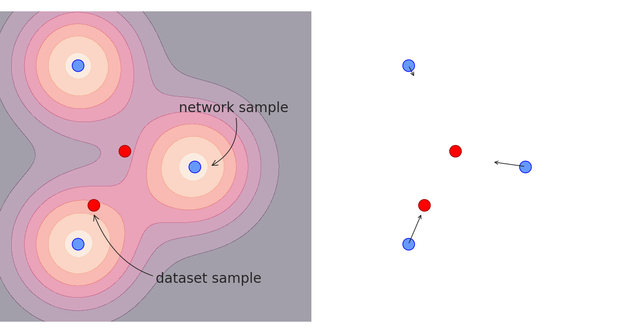
For example, suppose we have a large amount of samples \(z_j\) from \(Z\) and samples \(x_i\) from \(X\). We can check how we should change \(f_\theta(z_j)\) to increase the empirical log-likelihood.

with \(r_{ij} = x_i - f_\theta(z_j), \boldsymbol{d}_{ij} = \|r_{ij}\|_2\) and

In other words, each dataset sample is mainly pulling the closest (or the few closest) network samples. With a bigger variance, the softmin becomes less pronounced, so samples that are farther away start to get a bigger and bigger proportion of the pull. That is, bigger variance leads to a larger range but reduced “precision”.

Note that gaussian distributions with fixed variance are not the only possible distribution we can use. This is just an easy-to-understand example. Real VAEs tend to use more complicated distributions (see here), but the idea remains the same: let the network output some distribution that works as a training signal instead of using a single point.

How to approximate the log-likelihood

This takes care of the problem of the training signal, but we still need to solve a more important issue. How do we approximate the log-likelihood? A natural answer would be by sampling the generator, however that’s not a good idea.

As an analogy for what’s going on here let’s picture the following: You and a friend each have a deck of cards. Normally you would use these decks for some very elaborate card game. Each of your cards has all sorts of complicated effects on the behavior of the game. Your friend’s cards don’t need to be the same as yours, although you may have some cards in common or with similar behavior. So, your friend picks ten random cards from her deck and shows them to you⁶. How likely are you to get something like this? How can you estimate this efficiently?

A possible approach is taking a bunch of one-card samples from your deck. With this, you can estimate the probability of getting each of the individual cards from your friend’s hand (or something similar). Then you can combine the results by multiplying the probabilities, and you are done. Notice that your sampling procedure involves picking cards at random from a large deck and counting the appearances of things you were looking for. The downside with this method is that it is going to be really inefficient provided that the deck has enough diversity. Estimating the probability of a rare event by sampling is hard because, well, because it’s rare.

Ideally, we would like to sample from a distribution such that the event whose probability we are trying to approximate is a fairly common one. That’s the main idea. We would like to sample from a (hopefully) “easier” distribution. Of course, if we don’t use the original distribution then our estimated probabilities are not going to match exactly with the ones we truly want. We are gaining some efficiency but at the cost of having a biased estimate

Going back to our problem, we want to estimate the probability of observing dataset sample \(x\) when sampling the generator.

which we can approximate by sampling \(Z\) and using \(\frac{1}{n} \sum_i p_\theta(x \mid z_i)\). As we just saw, estimating \(p_\theta(x)\) by using this kind of sampling can still be really expensive because it may be rare to get a \(z\) that significantly contributes to the probability. So, we are going to modify the way we sample so that it depends on \(x\).

Before getting any further, we introduce a bit more notation.

• \(q_\phi(z \mid x)\) is going to be the parametrized distribution that we are going to sample from and we use \(\hat{Z}\) for the random variable associated with this distribution.
• We use \(p_\theta(z \mid x)\) to refer to the conditional probability that \(z\) was the one that produced \(x\). Hopefully context will make clear if we are talking about \(p_\theta(z\mid x)\) or \(p_\theta(x \mid z)\)

Now we are going to derive a useful property. Take the KL-divergence between both distributions.

By Bayes’s rule, we have:

So we can expand the right side to get

We rearrange the terms and get

So we can estimate \(\log p_\theta(x)\) by sampling any distribution that we want. This is not without a few setbacks

1. We don’t know \(D_{KL}[q_\phi(\cdot\mid x) \| p_\theta(\cdot\mid x)]\) and
2. \(D_{KL}[q_\phi(\cdot \mid x) \| u]\) can only be known analytically if both \(q_\phi(\cdot\mid x)\) and \(u\) are “easy”. Otherwise, we must estimate it via sampling.

The VAEs approach is to ignore \(D_{KL}[q_\phi(\cdot\mid x) \| p_\theta(\cdot\mid x)]\) and simply use the right side of the equation. This ends up as a lower bound on the log-probability of \(x\)

called evidence lower bound (ELBO), with equality only if \(q_\phi(\cdot \mid x)\) and \(p_\theta(\cdot \mid x)\) are the same ⁷. So, instead of maximizing the log-likelihood of the dataset, we try to maximize the expected value of the right side of the equation:

As we want to increase the bound as much as possible, we should optimize both on \(\theta\) and on \(\phi\). Assuming that \(\phi\) and \(\theta\) are flexible enough, as we start doing gradient ascent, \(q_\phi(\cdot \mid x)\) will start to resemble \(p_\theta(\cdot \mid x)\). However, if \(q_\phi\) can imitate any complicated distribution then we are also in trouble: how are we going to know \(D_{KL}[q_\phi(\cdot \mid x) \| u]\) analytically?

An assumption on \(q_\phi\)

In VAEs we usually decide to use \(q_\phi\) and \(u\) so that \(D_{KL}[q_\phi(\cdot \mid x) \| u]\) is easy to compute⁸. That’s a big assumption, we hope that it leads to a good enough lower bound. This is generally done by making them gaussian distributions. Here \(\phi\) is going to be a neural network that takes \(x\) and outputs the mean and variance, so \(\hat{Z} \mid x \sim \mathcal{N}(\mu_\phi(x),\Sigma_\phi(x))\). Similarly, \(u\) is going to be the standard gaussian distribution, so \(Z\sim \mathcal{N}(0,I)\). The main idea here is that we hope \(\theta\) is going to do most of the legwork by maximizing the lower bound while simultaneously keeping \(p_\theta(\cdot \mid x)\) approximately gaussian (or whatever distribution we decide to use).

Reparametrization trick

Something that may not be obvious at first is that we need to be a little bit careful about our sampling procedure for estimating \(\mathbb{E}_{\hat{Z} \sim q_\phi(\cdot \mid x)} [\log p_\theta(x \mid \hat{Z})]\). Suppose we do it by taking samples \(\hat{z}_i \sim q_\phi(\cdot \mid x)\) and then approximating the expected value using \(\frac{1}{n} \sum_i \log p_\theta(x \mid \hat{z_i})\). We won’t be able to backpropagate to \(\phi\). The problem is that the samples don’t give you any information about how \(\phi\)’s output interacts to produce this distribution. You are only seeing the final result. In the end, what’s \(\nabla_\phi \hat{z}_i\)?

The solution is decomposing the sampling as a function of \(\phi\)’s output and a random source (from a known and fixed distribution). That is \(\hat{z}_i = g(\text{output}_\phi(x), h_i)\) with \(h_i\) a sample from some distribution. Now \(\nabla_\phi \hat{z}_i\) makes sense.

As an example, for gaussian distributions we may use \(\hat{z}_i = \mu_\phi(x) + \Sigma_\phi(x)\epsilon_i\) with \(\epsilon_i\) sampled from \(\mathcal{N}(0,I)\)

An interpretation of the objective using KL-divergence

Here is an interesting view that might help us understand what are we really trying to maximize.

• First, take \((X,\hat{Z})\) to be the pair of random variables with the corresponding distributions. To get a sample from this pair you would first sample \(X\) and then you would sample \(\hat{Z}\) from the conditional given by \(q_\phi\).
• Similarly, take \((\hat{X},Z)\). Here you would sample from \(Z\) and then from the conditional given by \(p_\theta\).

Notice that \(X\) and \(Z\) have given distributions while:

• The \(\hat{Z}\)-distribution is determined by \(\phi\)
• The \(\hat{X}\)-distribution is determined by \(\theta\)

By playing a little with the equation of the objective we get that what we are actually optimizing is :

We changed the notation regarding KL-divergence in order to keep things short and to the point. \(D_{KL}[ X,\hat{Z} \| \hat{X},Z ]\) is the divergence between the associated distributions of both random variables. The entropy of \(X\) is a constant, we can ignore it so our optimization objective is:

We should also note that, originally, we wanted to maximize the log-likelihood of the dataset, this is equivalent to maximizing \(-D_{KL}[ X \| \hat{X}]\). In other words, regarding the objective used for optimization:

An interpretation as training a fuzzy autoencoder

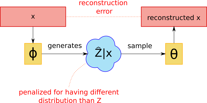
There is also a way to interpret this in an autoencoder context. Let’s assume, following a previous example, that \(p_\theta(x \mid z)\) is a gaussian with mean \(f_\theta(z)\) and fixed variance. In that case the logarithm is the square error multiplied by a constant associated with this variance⁹ (plus some constants). So, given the distribution \((X,\hat{Z})\), we are actually maximizing:

which we can interpret as a sort of “fuzzy” autoencoder. Here, \(\phi\) is trying to encode the value of \(X\) to a value of \(\hat{Z}\) in a non-deterministic fashion and \(\theta\) is trying to recover the original value of \(X\). There’s also a penalty involved if the process of generating \(\hat{Z}\) from \(X\) deviates too much from sampling from \(u\). This means that \(\phi\) is not allowed to do an arbitrarily good encoding. It needs to strike a balance between the autoencoder error and the regularization term.

We can see that the variance decides how important the regularization term should be. A large variance will prioritize making the distribution similar to \(u\) over transmitting any information about \(x\). On the other hand, a small variance will make \(\phi\) only care about it being possible to reconstruct \(x\) from \(\hat{z}\) even if the distribution looks nothing like \(u\). This may also lead to recovering traditional autoencoders provided that \(\phi\) is able to produce deterministic distributions.

Note that this interpretation of “VAEs as reconstruction loss + regularization” also holds for more complicated \(p_\theta(x \mid z)\) distributions. Although these are not as revealing as the relation between mean square error and the gaussian with fixed variance.

Is \(q_\phi\) really more efficient?

Remember that we introduced \(q_\phi\) hoping that it’s more sample efficient than sampling directly from \(u\). As \(q_\phi\) is ultimately trying to get close to \(p_\theta(\cdot \mid x)\) let’s assume that they are equal. The question now is, which is more sample efficient to estimate on average?

• Take \(K_l = \log \frac{1}{n}\sum p_\theta(X \mid Z_i)\) to be our estimator for the left side
• Take \(K_r = \frac{1}{n}\sum \log p_\theta(X \mid \hat{Z}_{i \mid X})\) to be our estimator for the right side

Intuitively it makes sense to think that, for the same \(n\), \(K_r\) has a smaller approximation error on average. However, is there a way to prove that it’s true? More precisely, does this estimator have a smaller, let’s say, mean square error?

I have no idea if there is any theorem about it. Is it true in general? If not, under what type of distributions can we guarantee that the property holds?

A vanilla implementation

Finally, we do a simple implementation of a VAE for image generation. You can see the details here. The architecture is nothing fancy. Through trial and error we ended up with something that looks like this:

With our final distribution being a gaussian with fixed variance. Does batch normalization help at all? Is a latent representation of 1024 unnecessarily big? I don’t have any answers for these questions but this architecture seems to work so if it ain’t broke…

We trained our network on the 128x128 version of the FFHQ dataset. The hardest part is finding a good balance between the mean square error and the KL-penalty. We ended up with a \(10^{-4}\) fraction of the loss coming from the KL-penalty and the rest from the square error. The samples look like this:

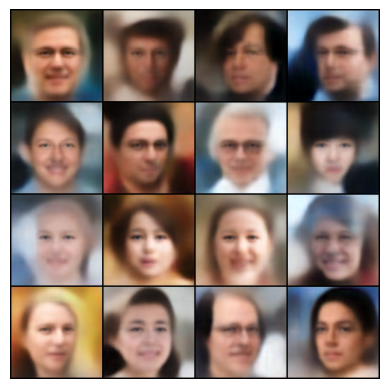
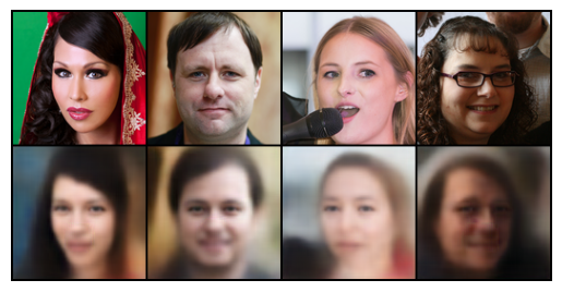
As you can see, the outputs are blurry. Looking back, this is probably due to the fact that we used a fixed variance, which is a really bad idea.

References

• Carl Doersch. 2016. Tutorial on Variational Autoencoders
• Diederik P Kingma, Max Welling. 2013. Auto-Encoding Variational Bayes

Footnotes